Examining the Effect of Ancillary and Derived Geographical Data on Improvement of Per-Pixel Classification Accuracy of Different Landscapes

Abstract

l

Introduction

l

Study Area and Data

l

Results and Discussion

l

Conclusion

l

Acknowledgement

l

References

Study Area and Data

3.1. Urban Classification: Greater Bangalore

The study area selected for urban classification is a part of the city of Greater Bangalore as seen in Google Earth image in Fig. 1a). The area in the scene is highly urbanised with the central business district. It consists of highly contrasting and heterogeneous features—race course (asoval shape in the first quadrant of the image), bus stand with semi-circular platforms, railway station with railway lines in the second quadrant, a park below the race course, dense builtup with concrete roofs, and some buildings with asbestos roofs, blue plastic roofs (one in the vicinity of the race course and 2 near the railway lines), tarred roads with flyovers, vegetation and few open areas (such as play ground, walk ways and vacant land). Dense and medium urban areas have high surrounding temperature compared to vegetation patches, parks and lakes (Ramachandra and Kumar 2009). The undulating terrain in the city ranges from 735 to 970 m with varying textures due to different urban structures. For this terrain two different data sets were used for the demonstration of urban classification— IKONOS MS and Landsat ETM + MS.

Fig. 1 a Part of greater Bangalore City as seen in Google Earth (left) and IKONOS image (right) IKONOS data along with ancillary and derived layers such as elevation, slope, NDVI, EVI and textures (ASM—angular second moment, contrast, entropy and variance) were used in separate experiments during classification as summarised in Table 1. In another set of experiments, Landsat ETM + data with 6 MS bands (resampled to 15 m) along with geographical layers, PAN and texture measures from PAN band making the total number of geographical layers to 125, were used in the classification as summarised in Table 2.

Table 1 Details of geographical layers used for IKONOS data classification

Table 2 Details of data and ancillary layers for Landsat ETM + MS classification of Bangalore City

3.2. Forested Landscape with Undulating Terrain: Case Study of Uttara Kannada District, Central Western Ghats

This region has gentle undulating hills, rising steeply from a narrow coastal strip bordering the Arabian sea to a plateau at an altitude of 500 m with occasional hills rising above 600–860 m. Climatic conditions range from arid to humid due to physiographic conditions ranging from plains, mountains to coast. Seven classifications were carried out with different combinations of Landsat ETM+ bands and geographical layers (such as temperature, elevation, EVI, slope, aspect, PAN and texture i.e. contrast and variance as listed in Table 3) into agriculture, builtup, forest, plantation, wasteland and water bodies that are the six major land use categories in the forested and mountainous terrain of Uttara Kannada district (Fig. 1b). The total number of geographical layers were altogether 65 as shown in Classification No. 7 in Table 3 which included Landsat ETM+ bands 1–5 and 7, temperature, EVI, PAN and texture (contrast and variance computed at 0, 45, 90 and 135 degrees on ETM? bands 1–5, 7 and ETM+ PAN band).

Fig.1b location of the study area in Central WesternGhats

Table 3 Details of data and ancillary layers for Landsat ETM + MS classification for a part of Central Western Ghats

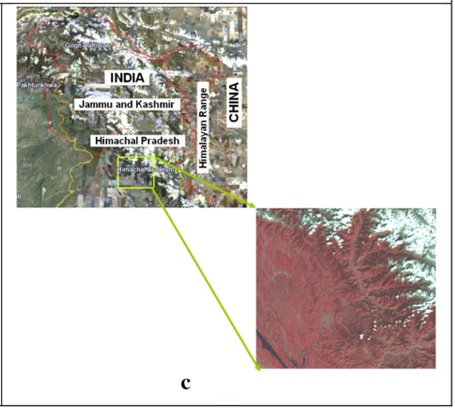
3.3. Mountainous Terrain in Temperate Climate: Mandhala Watershed, Western Himalaya

Mandhala watershed falls in lower Shivalik range of the Himalayas (Fig. 1c), dominated by dry evergreen tree species. This region is characterised by rugged terrain of Western Himalaya with altitude ranging from 295 to 6619 m above mean sea level. Nine different classification with combinations of Landsat ETM+ spectral bands, PAN and ancillary layers (viz. temperature, elevation, EVI, slope, aspect and texture) were carried out into four categories—vegetation, water, snow and others (settlement, rock, barren). In Classification No. 8, the combination of Landsat ETM+ bands, temperature, EVI and texture produced the highest number of input layers i.e. 104 (Table 4). Finally in Classification No. 9, only original spectral bands and their texture measures were considered (temperature and EVI layers were ignored) to make the total number of input layers in classification to 102 as seen in Table 4.Itis to be noted that high spatial resolution IKONOS data were not available for forested landscape in Western Ghats and for the Himalayan terrain.

Fig.1c location of study area in Western Himalaya (colour figure online)

Table 4 Details of data and ancillary layers for Landsat ETM + MS classification in Western Himalaya

The classifications were performed using RF which uses bagging to form an ensemble of classification tree. At each splitting node in the underlying classification trees, a random subset of the predictor variables is used as potential variables to define split. In training, it creates multiple Classification and Regression Tree trained on a boot- strapped sample of the original training data, and searches only across randomly selected subset of the input variables to determine a split for each node. The output of the classifier is determined by a majority vote of the trees that result in the greatest classification accuracy. It is superior to many tree-based algorithms, because it lacks sensitivity to noise and does not overfit. The trees in RF are not pruned; therefore, the computational complexity is reduced. As a result, RF can handle high dimensional data, using a large number of trees in the ensemble (Breiman and Cutler 2010). All the experiments were carried out on a Desktop computer with Intel Pentium IV processor, 3.00 GHz clock speed and 3.5 Gb RAM in Linux with GRASS GIS and R statistical package.

E-mail   |   Sahyadri   |   ENVIS   |   GRASS   |   Energy   |   CES   |   CST   |   CiSTUP   |   IISc   |   E-mail